Example Study Report - Group Sequential Design with Multiple Testing

2026-05-29

Introduction

With a 28-month accrual period, the total sample size planned for the study is 600.

Enrollment

• Piece-wise Constant Enrollment Rates
• Cumulative Enrollment

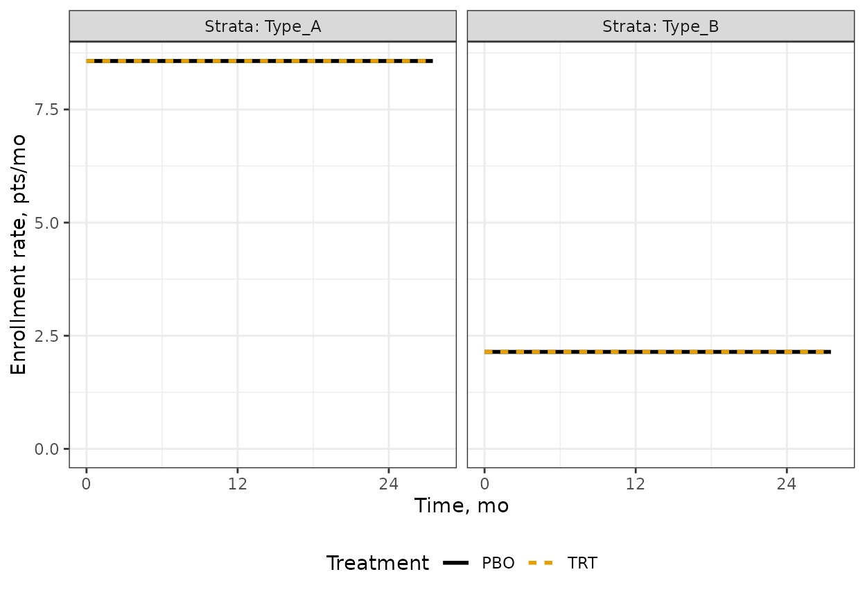
Multiplicity Adjustment

The multiplicity strategy follows the graphical approach for group sequential designs of Maurer and Bretz (2013) which provides strong control of type 1 error. The procedure takes into account both sources of multiplicity: multiple hypothesis tests (e.g., across primary and secondary endpoints) and multiple analyses planned for the study (i.e., interim and final analyses).

There are two key components that define this approach:

• Testing algorithm for multiple hypotheses specified by the graphical representation
• Repeated testing of some hypotheses using the alpha-spending function methodology

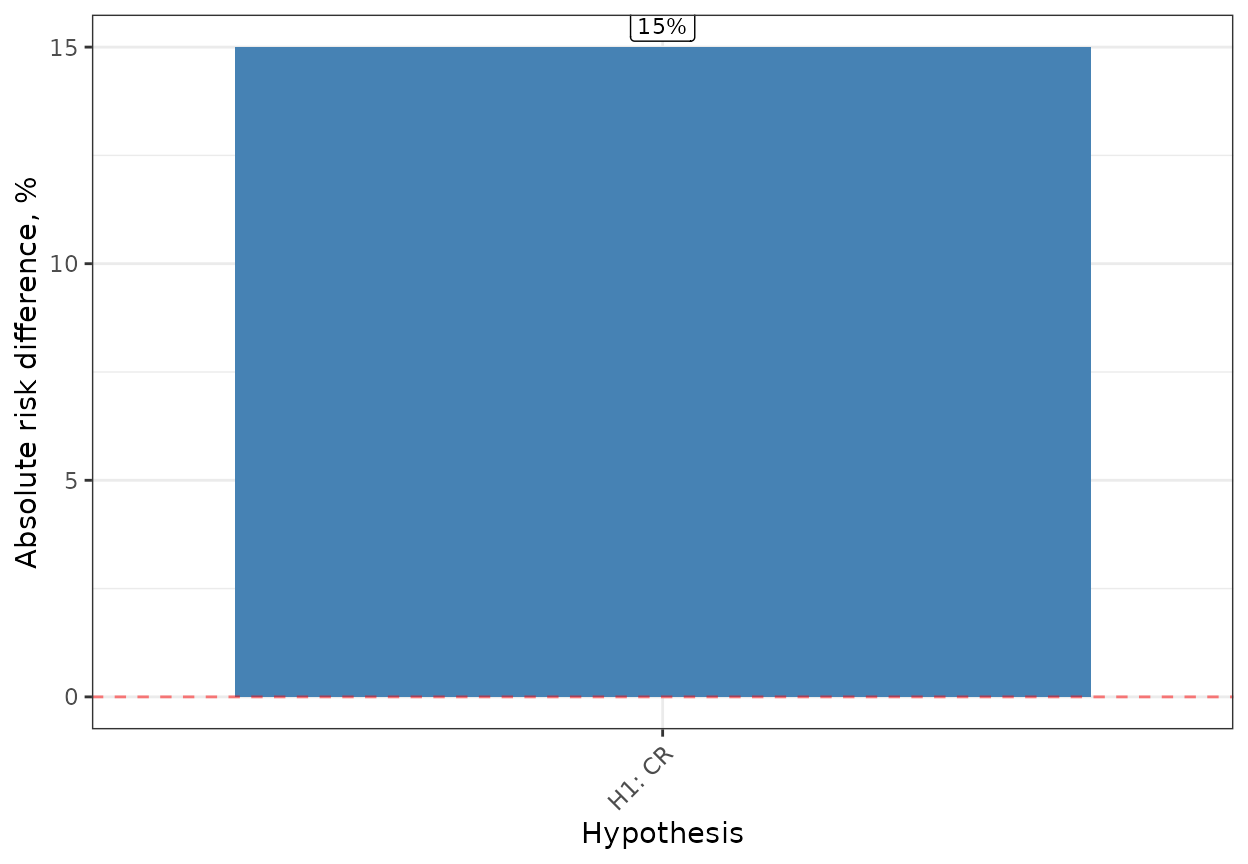
The multiplicity strategy will be applied to the 3 hypotheses across CR, OS, EFS endpoints. The following table summarizes the hypotheses specifying alpha-spending functions (for hypotheses to be tested group sequentially) together with the effect sizes and planned maximum statistical information (sample size or number of events).

Table 1. Summary of Primary and Key Secondary Hypotheses

Trial Design Summary

Label	Endpoint	Type	Initial weight	GSD spending fn	Effect size*	Maximum events / sample size
H1	CR	Primary	0.4	N/A	Delta = 15%	500
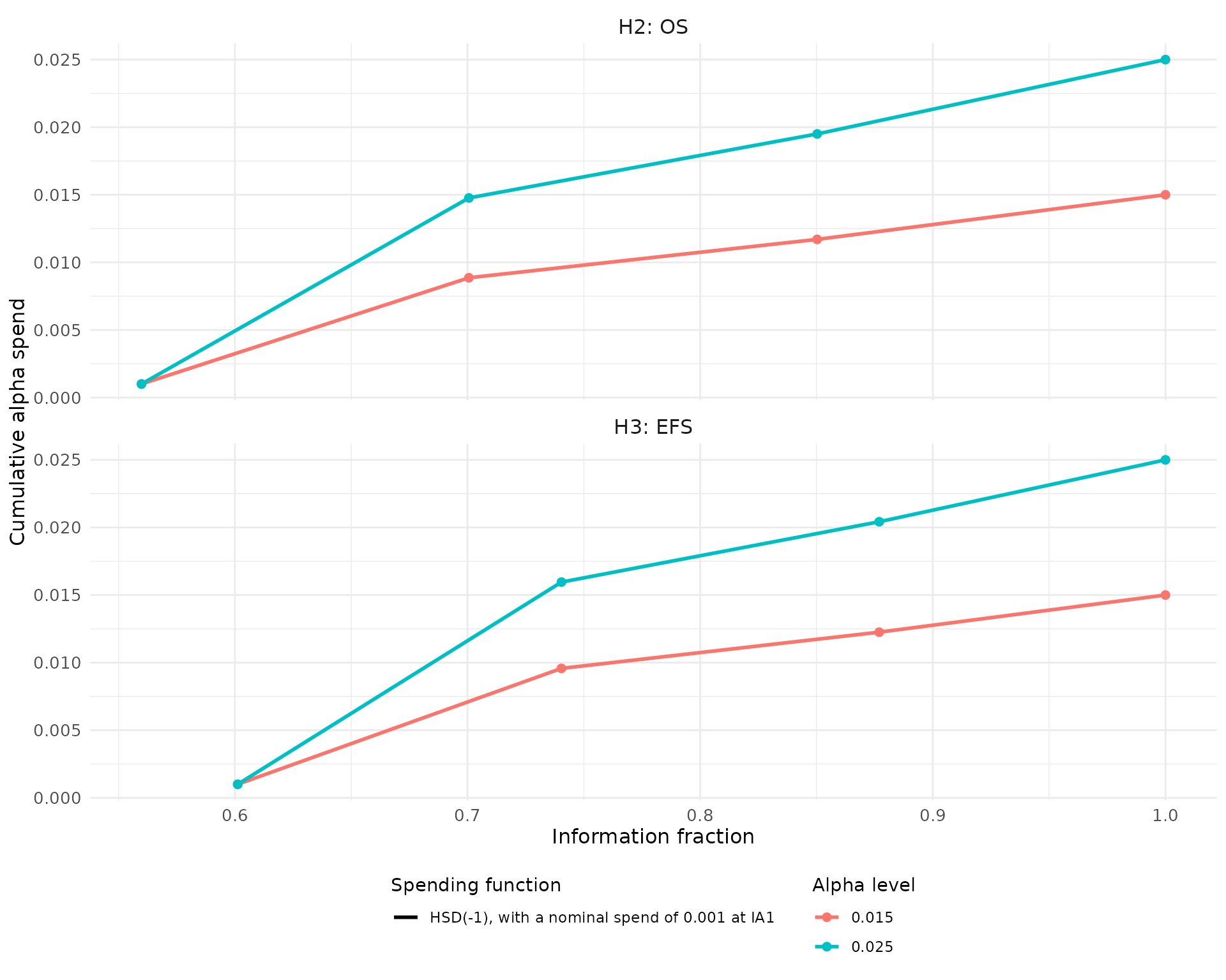
H2	OS	Primary	0.6	HSD(-1), with a nominal spend of 0.001 at IA1	HR = 0.69	334
H3	EFS	Secondary	0	HSD(-1), with a nominal spend of 0.001 at IA1	AHR = 0.68	413
*For a hypothesis corresponding to a time-to-event variable subject to non-proportional hazards, the listed effect size is the average hazard ratio at the final analysis of this hypothesis.

The overall type I family-wise error rate for 3 hypotheses, over all (interim and final) analyses, is controlled to 2.5% (one-sided).

Distribution Assumptions

• Binary Endpoints
• Time-to-Event Endpoints

Rates

Absolute Risk Differences

Drop-out Rates

Cumulative Drop-out Probabilities

Hazard Rate

Cumulative Hazard

Survival Curves

Median Survival

Survival Quantiles

Enrollment Weighted Survival Curves

Piece-wise Hazard Ratios

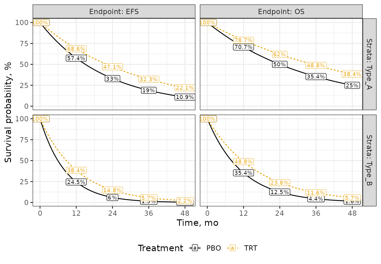
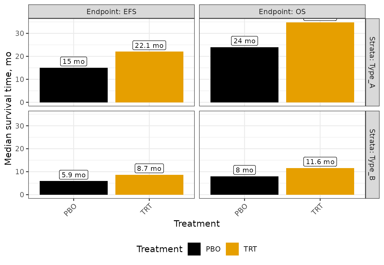
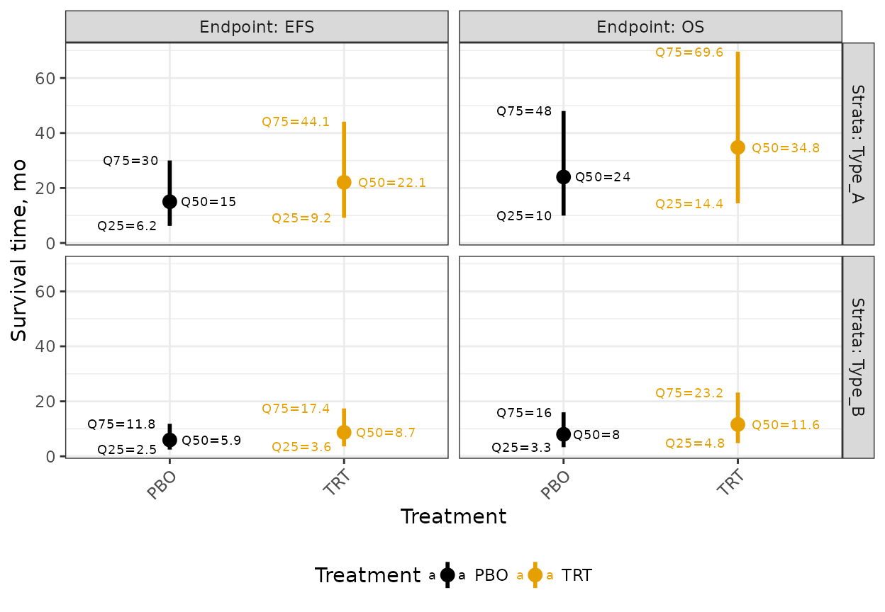
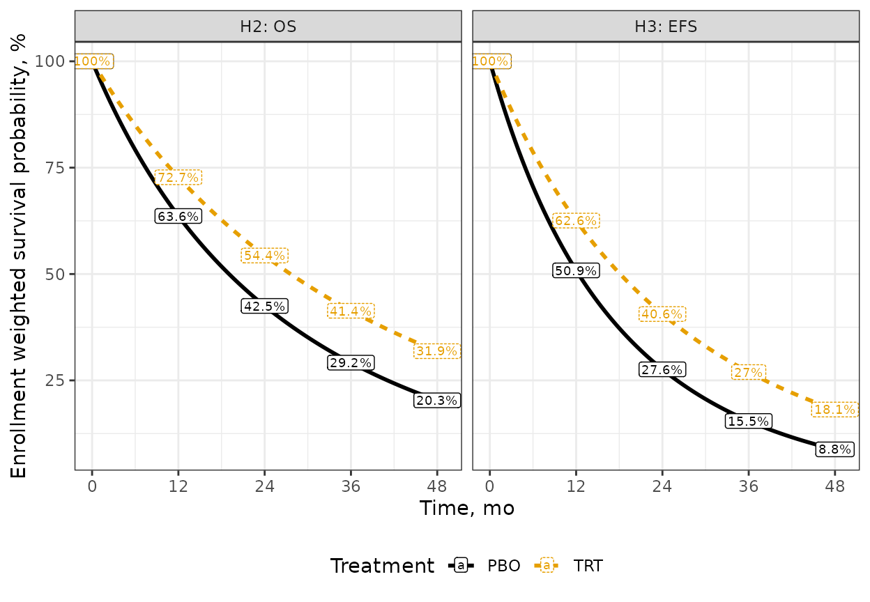
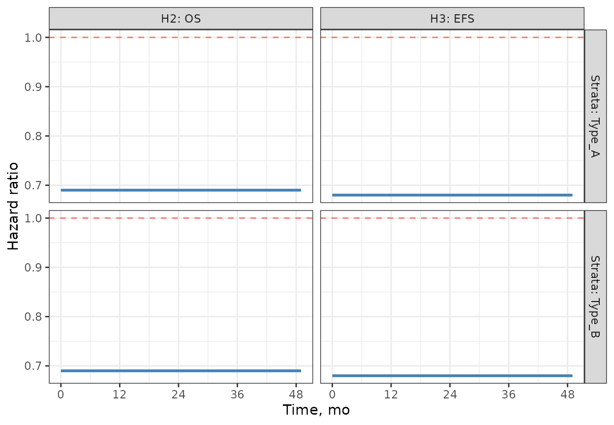
Average Hazard Ratios

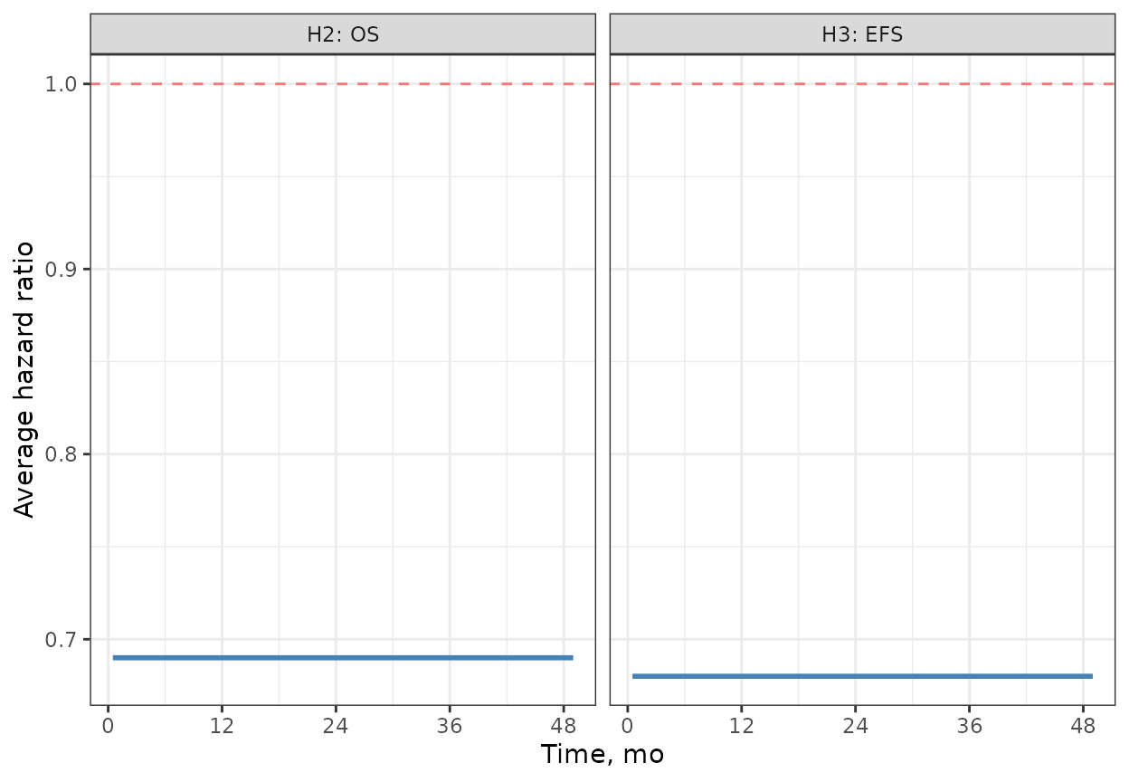
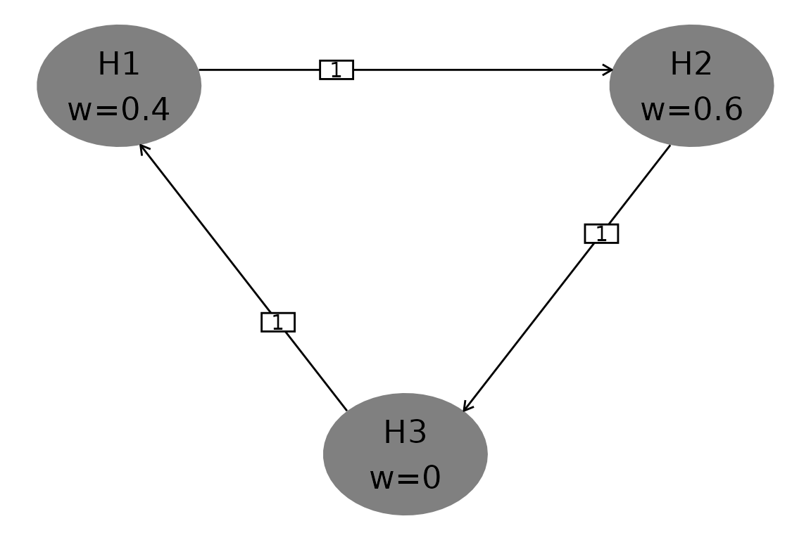
Figure 1 shows the graph where the hypotheses of interest are represented by the elliptical nodes. Each node has the hypothesis weight assigned to it (denoted by $w$). A particular value of $w$ sets the local significance level associated with that hypothesis (which is equal to 0.025 × $w$). The graphical approach allows local significance levels to be recycled (along arrows on the graph) when a given hypothesis is successful (i.e., the corresponding null hypothesis is rejected) at interim or final analyses.

Figure 1. Graph Depicting Multiple Hypothesis Testing Strategy

Interim Analyses

• IA by Hypothesis
• IA by Calendar Time
• Information Flow
• Timeline of Planned Analyses

Table 2. Summary of Interim Analyses (by hypotheses)

Summary of interim analyses by hypothesis

Analysis	Criteria for conduct	Events / sample size	Expected analysis time, mo	Information fraction, %
H1: CR
1	500 CR outcomes	500	28.0	100.00%
H2: OS
1	500 CR outcomes	187	28.0	55.98%
2	234 OS events	234	32.8	70.06%
3	284 OS events	284	39.4	85.03%
4	334 OS events	334	48.7	100.00%
H3: EFS
1	500 CR outcomes	248	28.0	60.12%
2	234 OS events	306	32.8	74.04%
3	284 OS events	362	39.4	87.70%
4	334 OS events	413	48.7	100.00%

Table 3. Summary of Interim Analyses (by calendar analysis)

Summary of interim analyses by criteria for conduct

Hypothesis	Analysis	Events / sample size	Information fraction, %
500 CR outcomes (Expected analysis time: 28.0 mo)
H1: CR	1	500	100.00%
H2: OS	1	187	55.98%
H3: EFS	1	248	60.12%
234 OS events (Expected analysis time: 32.8 mo)
H2: OS	2	234	70.06%
H3: EFS	2	306	74.04%
284 OS events (Expected analysis time: 39.4 mo)
H2: OS	3	284	85.03%
H3: EFS	3	362	87.70%
334 OS events (Expected analysis time: 48.7 mo)
H2: OS	4	334	100.00%
H3: EFS	4	413	100.00%

Figure 2. Information Factor Over Time by Hypothesis

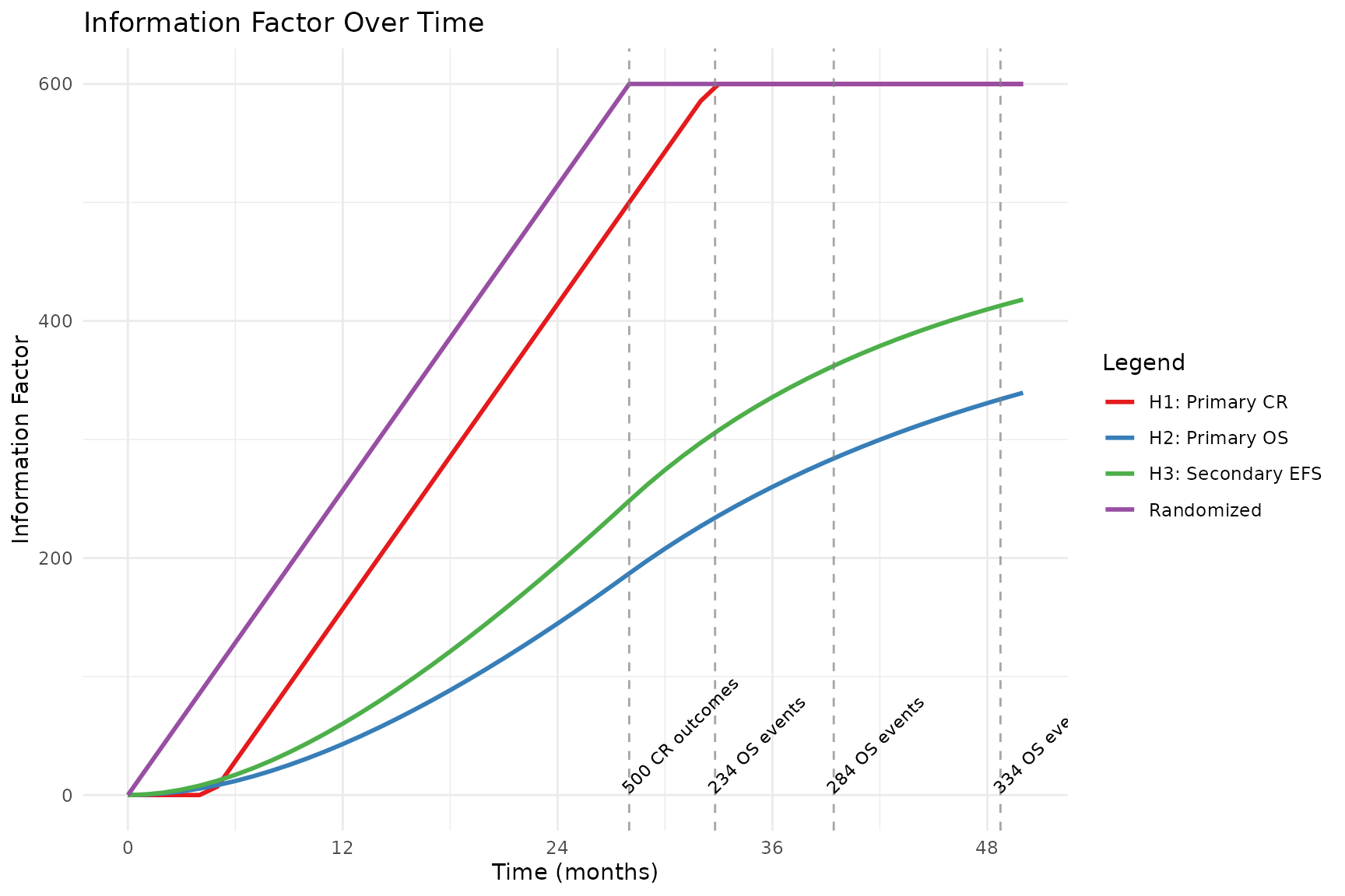
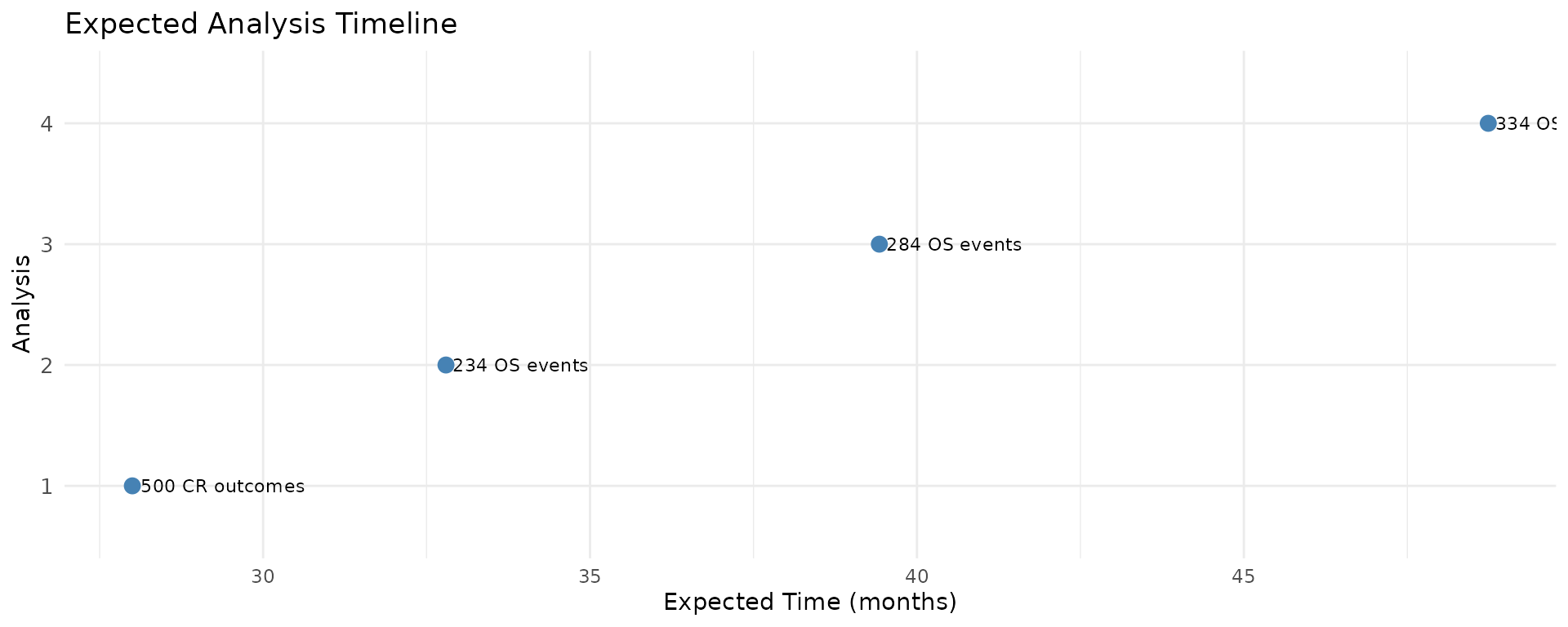
Figure 3. Anticipated study timeline

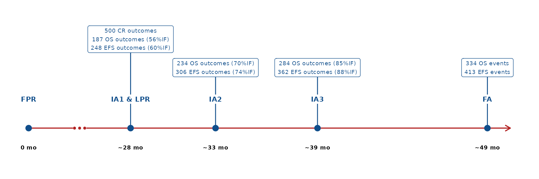
Figure 3b. Anticipated time of each analysis, with associated trigger

Hypothesis Testing

• Scenarios
• Boundary Specifications
• Operating Characteristics by Analysis
• Operating Characteristics Overall
• Spending Functions

Table 4. Weight Allocation Scenarios

Summary of alpha allocation by hypothesis

Local alpha level	Weight	Testing scenario
H1: CR
0.01000	0.4	Initial allocation
0.02500	1	Successful H2, H3
H2: OS
0.01500	0.6	Initial allocation
0.02500	1	Successful H1
H3: EFS
0.01500	0.6	Successful H2
0.02500	1	Successful H1, H2

Table 5. Boundary Specifications

Table 5 details the hypothesis testing at the interim and final analyses. For hypotheses tested group sequentially, the table provides the nominal p-value boundary derived from the alpha-spending function and the information fractions. The timing of analyses is expressed in terms of statistical information fractions. The table also reports local power at each analysis time.

Operating characteristics

Analysis	Local alpha level	Nominal p-value	Exit hurdle	Local power	Information fraction, %
H1: CR
1	0.01000	0.01000	0.104	85.551%	100.00%
1	0.02500	0.02500	0.088	92.379%	100.00%
H2: OS
1	0.01500	0.00100	0.636	29.177%	55.98%
2	0.01500	0.00876	0.733	68.021%	70.06%
3	0.01500	0.00717	0.748	78.351%	85.03%
4	0.01500	0.00848	0.770	86.995%	100.00%
1	0.02500	0.00100	0.636	29.177%	55.98%
2	0.02500	0.01472	0.752	74.783%	70.06%
3	0.02500	0.01251	0.766	84.062%	85.03%
4	0.02500	0.01493	0.788	91.232%	100.00%
H3: EFS
1	0.01500	0.00100	0.676	47.949%	60.12%
2	0.01500	0.00950	0.765	85.213%	74.04%
3	0.01500	0.00753	0.775	91.465%	87.70%
4	0.01500	0.00832	0.790	95.564%	100.00%
1	0.02500	0.00100	0.676	47.949%	60.12%
2	0.02500	0.01593	0.782	89.508%	74.04%
3	0.02500	0.01314	0.792	94.515%	87.70%
4	0.02500	0.01468	0.807	97.542%	100.00%

Table 6a. Operating Characteristics at Each Analysis

Operating characteristics by analysis

Analysis	Metric	Hypothesis subset	Probability, %
1	Power	H1	87.500%
		H2	29.000%
		H3	14.300%
	Probability of success for at least one Hi	H1, H2	90.700%
		H1, H2, H3	90.700%
	Probability of success for all Hi	H1, H2, H3	13.300%
2	Power	H1	89.900%
		H2	74.200%
		H3	66.300%
	Probability of success for at least one Hi	H1, H2	95.600%
		H1, H2, H3	95.600%
	Probability of success for all Hi	H1, H2, H3	62.200%
3	Power	H1	90.700%
		H2	84.200%
		H3	78.800%
	Probability of success for at least one Hi	H1, H2	96.900%
		H1, H2, H3	96.900%
	Probability of success for all Hi	H1, H2, H3	73.600%
4	Power	H1	91.900%
		H2	91.000%
		H3	87.400%
	Probability of success for at least one Hi	H1, H2	98.600%
		H1, H2, H3	98.600%
	Probability of success for all Hi	H1, H2, H3	81.200%

Table 6b. Operating Characteristics Across Analyses

Operating characteristics across analyses

Metric	Hypothesis subset	Value
Expected Success Analysis	H1	1.08
	H2	1.94
	H3	2.18
Expected Success Analysis (at least one Hi)	H1, H2	1.13
	H1, H2, H3	1.13
Expected Success Analysis (for all Hi)	H1, H2, H3	2.16
Expected Success Time	H1	28.5
	H2	33.2
	H3	34.5
Expected Success Time (at least one Hi)	H1, H2	28.7
	H1, H2, H3	28.7
Expected Success Time (for all Hi)	H1, H2, H3	34.4

Figure 4. Alpha-spending functions

Configuration Details

Graph Structure

Table 7. Transition Matrix

0	1	0
0	0	1
1	0	0

Initial Weights: 0.4, 0.6, 0

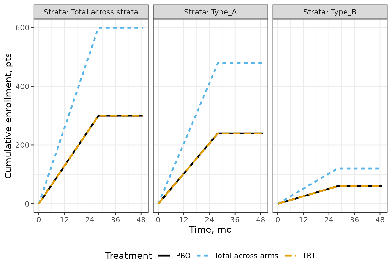
Enrollment Assumptions

Table 8. Enrollment Rate Assumptions

stratum	treatments	rate	duration	ratio
Type_A	PBO, TRT	17.14	28	1, 1
Type_B	PBO, TRT	4.29	28	1, 1

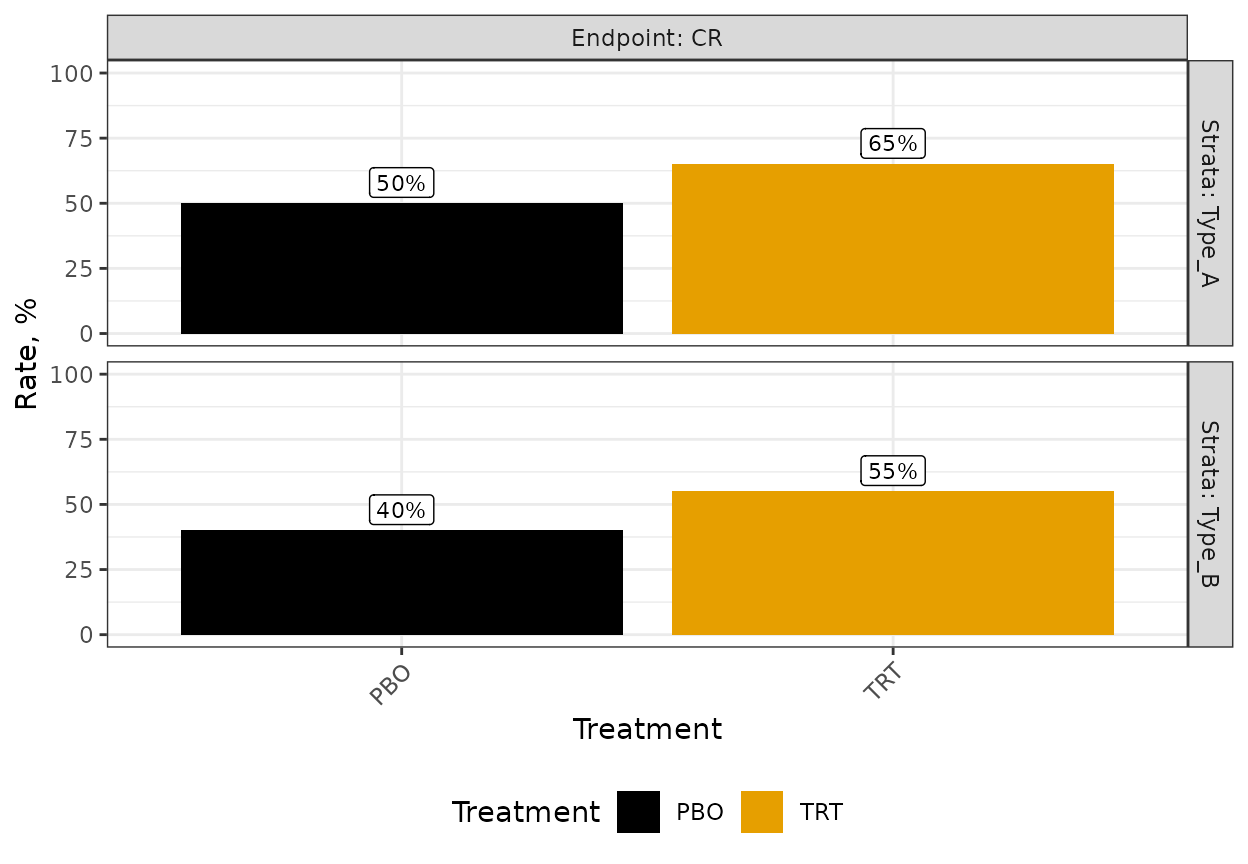
Binary Endpoint Assumptions

Table 9. Binary Endpoint Parameters

endpoint	stratum	treatment	rate	maturity_time
CR	Type_A	PBO	0.50	4.667
CR	Type_B	PBO	0.40	4.667
CR	Type_A	TRT	0.65	4.667
CR	Type_B	TRT	0.55	4.667

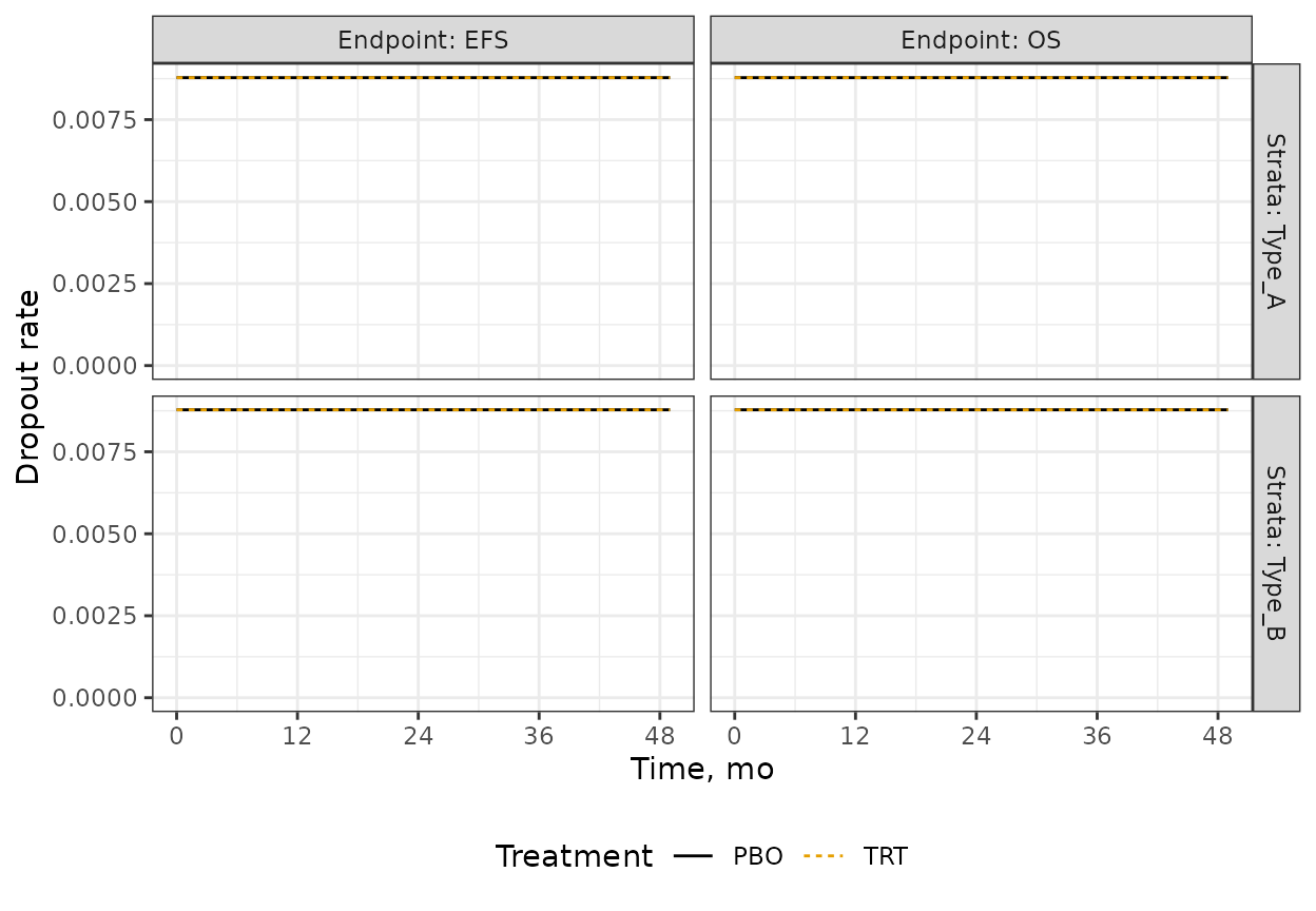
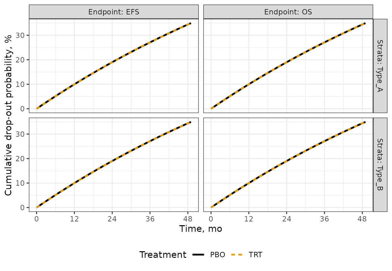
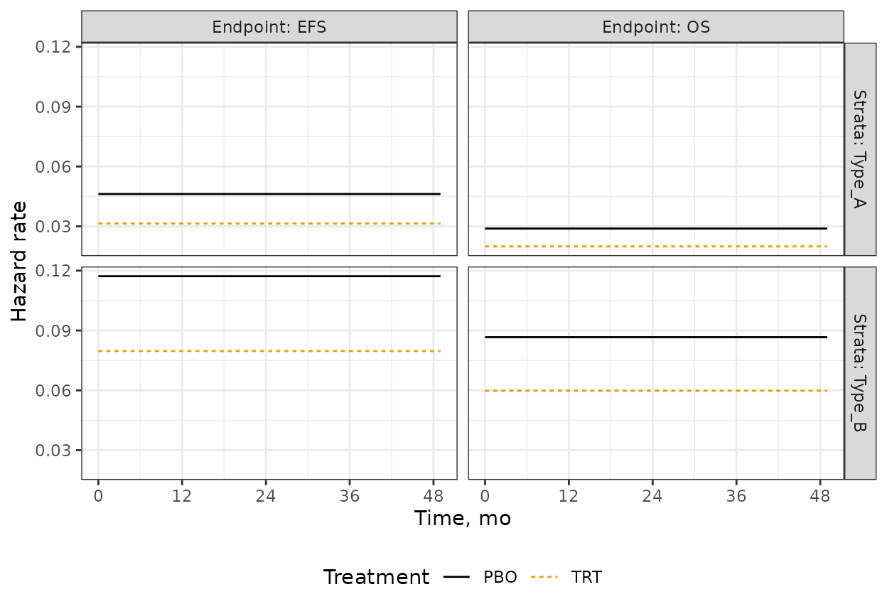
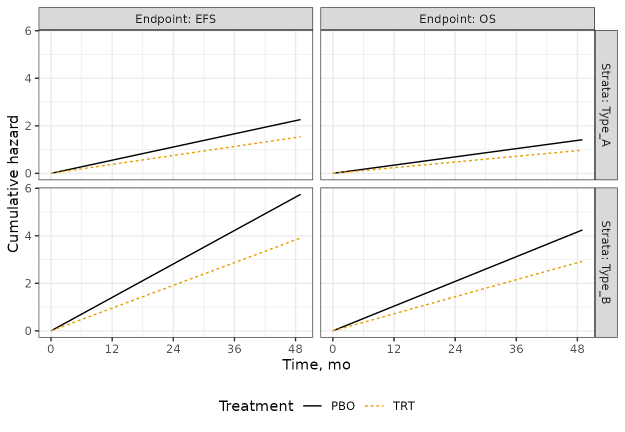
Time-to-Event Endpoint Assumptions

Table 10. Time-to-Event Distribution Parameters

endpoint	stratum	treatment	duration	fail_rate	dropout_rate
EFS	Type_A	PBO	Inf	0.0462	0.0088
EFS	Type_B	PBO	Inf	0.1172	0.0088
EFS	Type_A	TRT	Inf	0.0314	0.0088
EFS	Type_B	TRT	Inf	0.0797	0.0088
OS	Type_A	PBO	Inf	0.0289	0.0088
OS	Type_B	PBO	Inf	0.0866	0.0088
OS	Type_A	TRT	Inf	0.0199	0.0088
OS	Type_B	TRT	Inf	0.0598	0.0088

References

Maurer W, Bretz F. Multiple testing in group sequential trials using graphical approaches. Statistics in Biopharmaceutical Research. 2013;5(4):311-320.

---

Report generated on 2026-05-29 17:43:29.100101